How to sort data by multiple columns in Excel

Sorts are a simple task in Microsoft Excel if all you need is an ascending or descending sort. Excel is smart enough that it can interpret the data range. Not all sorts are so easy. Fortunately, Excel offers two types of custom sorts: by irregular terms and by multiple columns. The recent article, How to create a custom sort when a regular sort won’t do in Excel, shows you how to create a unique list of sorting elements, such as Monday, Tuesday and so on, or Small, Medium and Large. In this article, I’ll show you how to sort by multiple columns. For instance, you might want to sort a sales sheet by personnel and then region. The end result groups the personnel and then further groups each of those groups by region.

SEE: Excel tips every user should master (TechRepublic)

There are two ways to initiate a custom sort:

• On the Home tab, click Sort in the Editing group and click Custom Sort.
• On the Data tab, click Sort in the Sort & Filter group.

Please use whichever you prefer throughout the article.

I’m using Microsoft 365 on a Windows 10 64-bit system, but you can use older versions. For your convenience, you can download the demonstration .xlsx and .xls files. Excel Online supports sorting by multiple columns.

How to sort by two columns

Grouping is a common database task, and sorting by multiple columns is essentially the same thing. You have a primary sort on a specific column and then a secondary sort within the results of the primary sort. You’re not limited to two columns either, but we’ll keep the examples simple.

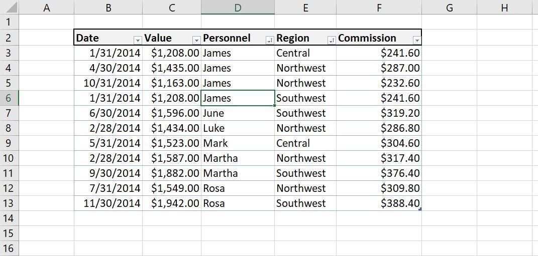
Figure A shows a simple data set of sales data for several people and the respective regions for each record. Let’s suppose you want to review the total commissions per personnel broken down by the regions. This requirement will need a sort by multiple columns; the primary sort will be on the Personnel column, and the secondary sort will be on the Region column.

Figure A

You can sort by personnel or region, but using the Sort options alone, you can’t sort by both. In this case, you need to build a custom sort as follows:

1. Click anywhere inside the data set, preferably in the Personnel column, but doing so isn’t necessary.
2. In the Editing group (on the Home tab), click the Sort & Filter option, and choose Custom Sort from the dropdown list.
3. If you clicked inside the Personnel column, the first Sort By setting in the result dialog should be Personnel. If you didn’t, choose Personnel now. The Sort On and Order options should be set to Cell Values and A To Z, respectively because these are the default settings. If necessary, make changes.
4. At this point, you’ve satisfied the primary sort. To build the secondary sort, click the Add Level option.
5. From the Then By dropdown, choose Region. Again, the Sort On and Order columns should be set to the defaults, Cell Values and A To Z (Figure A).
6. Now you have both sort columns set, so click OK to execute the sort.

As you can see in Figure B, Excel groups the names in the Personnel column in an ascending alphabetic sort. Then, the regions are sorted within each name group. James has three regions, Central Northwest, and Southwest. Then, drop down to Martha and Rosa. Their region groups are the same, Northwest and Southwest.

Figure B

This sort was rather easy. There are only two columns and they’re contiguous. Let’s complicate the requirements just a bit with a second example.

How to add a third column to sort in Excel

There are very few repeated dates, but there are a few repeated months. Let’s create a new custom sort on three columns: Date, Personnel and Region. To do so, we’ll first have to add a helper column—one that returns the month. To do so, insert a column between Date and Value, enter the following function in C3 and copy it to the remaining cells:

=Month(B3)

=Month([@Date]) (if you’re using a Table object)

Then, set the format to General. Doing so will display values that represent the month. For instance, 1 is January, 4 is April, 10 is October, and so on. Now, let’s set up a new custom sort:

1. Click anywhere inside the data set, preferably in the Date column, but doing so isn’t necessary.
2. In the Editing group (on the Home tab), click the Sort & Filter option, and choose Custom Sort from the dropdown list.
3. If you clicked inside the Date column, the first Sort By setting in the result dialog should be Date. If you didn’t before, choose Date now. The Sort On and Order options should be set to Cell Values and Oldest To Newest, respectively. If necessary, make those changes.
4. At this point, you’ve satisfied the primary sort. To build the secondary sort, click the Add Level option.
5. From the Then By dropdown, choose Personnel. Again, the Sort On and Order columns should be set to the defaults, Cell Values and A To Z.
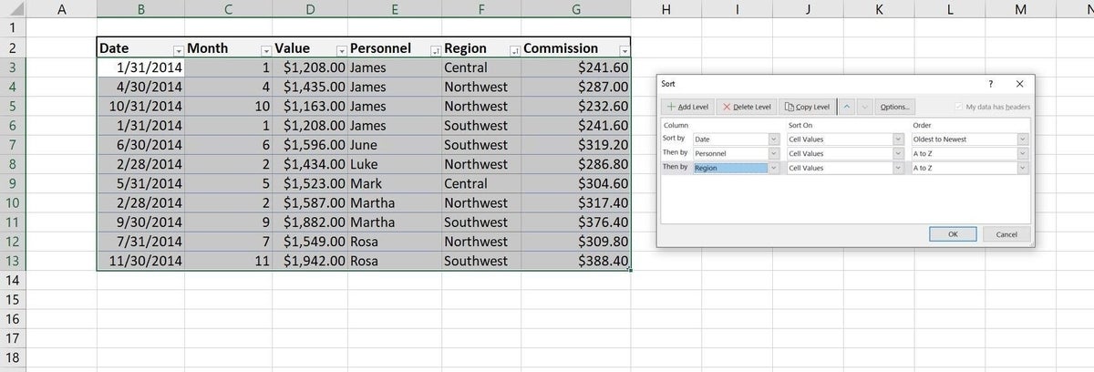
6. Click Add Level, choose Region from the Then By dropdown (Figure C), and click OK to execute the sort.

Figure C

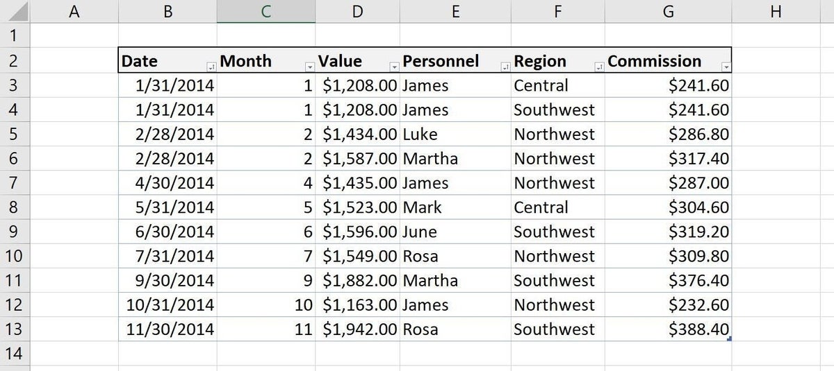
As you can see in Figure D, January 31 is the first date group. James is the only person with a sale in January, but he has two and the regions are alphabetically sorted. Luke and Martha are sorted within the February 28 group, and both have one region, Northwest.

Figure D

The data set is simple on purpose so you can easily discern the different groups as a result of the multiple column sorts. For each group, simply add a new sort level.